Compute and display similarities between multiple kernels

Compute cosine from Frobenius norm between kernels and display the corresponding correlation plot.

cim.kernel(
  ...,
  scale = TRUE,
  method = c("circle", "square", "number", "shade", "color", "pie")
)

Arguments

...: list of kernels (called 'blocks') computed on different datasets and measured on the same samples.
scale: boleean. If scale = TRUE, each block is standardized to zero mean and unit variance and cosine normalization is performed on the kernel. Default: TRUE.
method: character. The visualization method to be used. Currently, seven methods are supported (see Details).

Value

cim.kernel returns a matrix containing the cosine from Frobenius norm between kernels.

Details

The displayed similarities are the kernel generalization of the RV-coefficient described in Lavit et al., 1994.

The plot is displayed using the corrplot package. Seven visualization methods are implemented: "circle" (default), "square", "number", "pie", "shade" and "color". Circle and square areas are proportional to the absolute value of corresponding similarities coefficients.

References

Lavit C., Escoufier Y., Sabatier R. and Traissac P. (1994). The ACT (STATIS method). Computational Statistics and Data Analysis, 18(1), 97-119.

Mariette J. and Villa-Vialaneix N. (2018). Unsupervised multiple kernel learning for heterogeneous data integration. Bioinformatics, 34(6), 1009-1015.

Author

Jerome Mariette <jerome.mariette@inrae.fr> Nathalie Vialaneix <nathalie.vialaneix@inrae.fr>

Examples

data(TARAoceans)

# compute one kernel per dataset
phychem.kernel <- compute.kernel(TARAoceans$phychem, kernel.func = "linear")
pro.phylo.kernel <- compute.kernel(TARAoceans$pro.phylo, 
                                   kernel.func = "abundance")
pro.NOGs.kernel <- compute.kernel(TARAoceans$pro.NOGs, 
                                  kernel.func = "abundance")

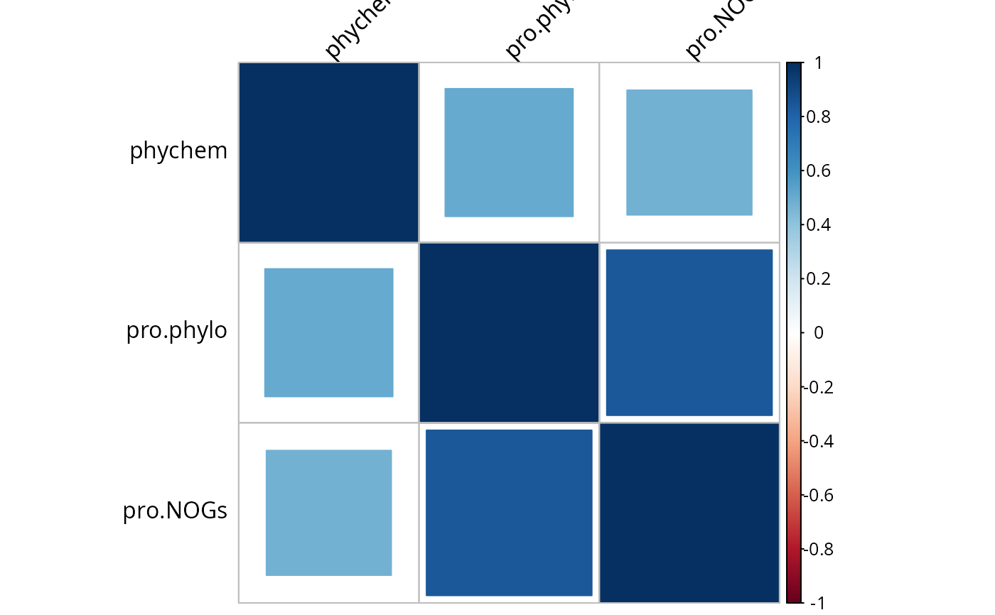
# display similarities between kernels
cim.kernel(phychem = phychem.kernel,
           pro.phylo = pro.phylo.kernel,
           pro.NOGs = pro.NOGs.kernel, 
           method = "square")