Data Integration using Unsupervised Multiple Kernel Learning
Jérôme Mariette, Céline Brouard, Rémi Flamary and Nathalie Vialaneix
25 avril, 2025
mixKernelUsersGuide.RmdIntroduction
The TARA Oceans expedition facilitated the study of plankton communities by providing ocean metagenomic data combined with environmental measures to the scientific community. This study focuses on 139 prokaryotic-enriched samples collected from 68 stations and spread across three depth layers: the surface (SRF), the deep chlorophyll maximum (DCM) layer and the mesopelagic (MES) zones. Samples were located in 8 different oceans or seas: Indian Ocean (IO), Mediterranean Sea (MS), North Atlantic Ocean (NAO), North Pacific Ocean (NPO), Red Sea (RS), South Atlantic Ocean (SAO), South Pacific Ocean (SPO) and South Ocean (SO).
In this vignette, we consider a subset of the original data analyzed in the article (Mariette & Villa-Vialaneix, 2018) and illustrate the usefulness of mixKernel to 1/ perform an integrative exploratory analysis as in (Mariette & Villa-Vialaneix, 2018) and to 2/ select relevant variables for unsupervised analysis.
The data include 1% of the 35,650 prokaryotic OTUs and of the 39,246 bacterial genes that were randomly selected. The aim is to integrate prokaryotic abundances and functional processes to environmental measure with an unsupervised method.
Install and load the mixOmics and mixKernel packages:
Loading TARA Ocean datasets
The (previously normalized) datasets are provided as matrices with matching sample names (rownames):
data(TARAoceans)
# more details with: ?TARAOceans
# we check the dimension of the data:
lapply(list("phychem" = TARAoceans$phychem, "pro.phylo" = TARAoceans$pro.phylo,
            "pro.NOGs" = TARAoceans$pro.NOGs), dim)
## $phychem
## [1] 139 22
##
## $pro.phylo
## [1] 139 356
##
## $pro.NOGs
## [1] 139 638Multiple kernel computation
Individual kernel computation
For each input dataset, a kernel is computed using the function
compute.kernel with the choice of linear, phylogenic or
abundance kernels. A user defined function can also be provided as
input(argument kernel.func, see
?compute.kernel).
The results are lists with a ‘kernel’ entry that stores the kernel matrix. The resulting kernels are symmetric matrices with a size equal to the number of observations (rows) in the input datasets.
phychem.kernel <- compute.kernel(TARAoceans$phychem, kernel.func = "linear")
pro.phylo.kernel <- compute.kernel(TARAoceans$pro.phylo, kernel.func = "abundance")
pro.NOGs.kernel <- compute.kernel(TARAoceans$pro.NOGs, kernel.func = "abundance")

# check dimensions
dim(pro.NOGs.kernel$kernel)
## [1] 139 139A general overview of the correlation structure between datasets is
obtained as described in Mariette and Villa-Vialaneix (2018) and
displayed using the function cim.kernel:
cim.kernel(phychem = phychem.kernel,
           pro.phylo = pro.phylo.kernel,
           pro.NOGs = pro.NOGs.kernel,
           method = "square")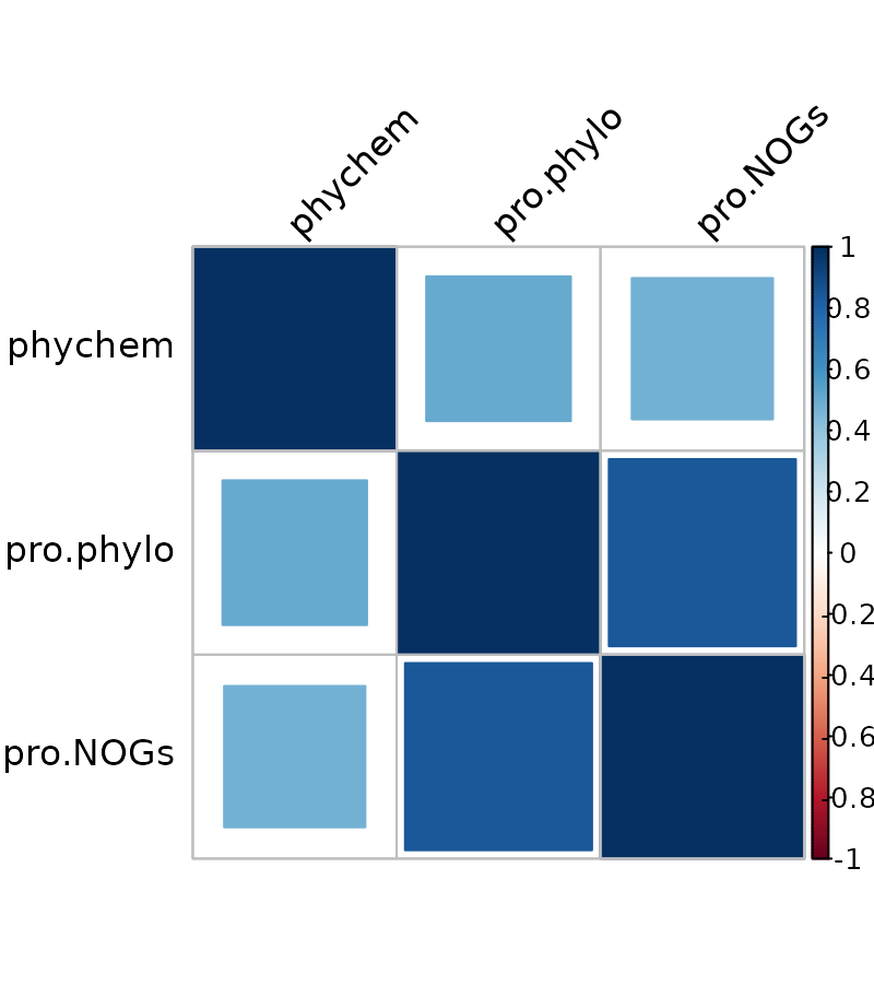
The figure shows that pro.phylo and
pro.NOGs is the most correlated pair of kernels. This
result is expected as both kernels provide a summary of prokaryotic
communities.
Combined kernel computation
The function combine.kernels implements 3 different
methods for combining kernels: STATIS-UMKL, sparse-UMKL and full-UMKL
(see more details in Mariette and Villa-Vialaneix, 2018). It returns a
meta-kernel that can be used as an input for the function
kernel.pca (kernel PCA). The three methods bring
complementary information and must be chosen according to the research
question.
The STATIS-UMKL approach gives an overview on the common
information between the different datasets. The full-UMKL
computes a kernel that minimizes the distortion between all input
kernels. The sparse-UMKL is a sparse variant of
full-UMKL that selects the most relevant kernels in
addition to distortion minimization.
meta.kernel <- combine.kernels(phychem = phychem.kernel,
                               pro.phylo = pro.phylo.kernel,
                               pro.NOGs = pro.NOGs.kernel,
                               method = "full-UMKL")
Exploratory analysis: Kernel Principal Component Analysis (KPCA)
Perform KPCA
A kernel PCA can be performed from the combined kernel with the
function kernel.pca``. The argumentncomp` allows to choose
how many components to extract from KPCA.
kernel.pca.result <- kernel.pca(meta.kernel, ncomp = 10)Sample plots using the plotIndiv function from
mixOmics:
all.depths <- levels(factor(TARAoceans$sample$depth))
depth.pch <- c(20, 17, 4, 3)[match(TARAoceans$sample$depth, all.depths)]
plotIndiv(kernel.pca.result,
          comp = c(1, 2),
          ind.names = FALSE,
          legend = TRUE,
          group = as.vector(TARAoceans$sample$ocean),
          col = c("#f99943", "#44a7c4", "#05b052", "#2f6395", "#bb5352",
                  "#87c242", "#07080a", "#92bbdb"),
          pch = TARAoceans$sample$depth,
          legend.title = "Ocean / Sea",
          title = "Projection of TARA Oceans stations",
          size.title = 10,
          legend.title.pch = "Depth")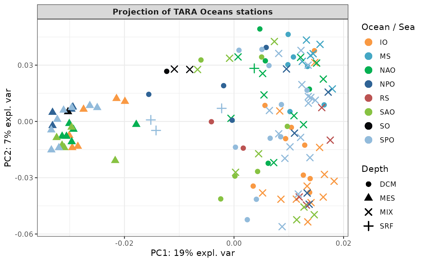
The explained variance supported by each axis of KPCA is displayed
with the plot function, and can help choosing the number of
components in KPCA.
plot(kernel.pca.result)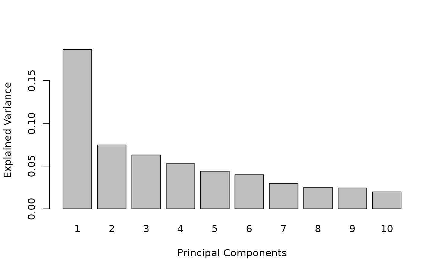
The first axis summarizes ~ 20% of the total variance.
Assessing important variables
Here we focus on the information summarized on the first component.
Variable values are randomly permuted with the function
permute.kernel.pca.
In the following example, physical variable are permuted at the
variable level (kernel phychem), OTU abundances from
pro.phylo kernel are permuted at the phylum level (OTU
phyla are stored in the second column, named Phylum, of the
taxonomy annotation provided in TARAoceans object in the
entry taxonomy) and gene abundances from
pro.NOGs are permuted at the GO level (GO are provided in
the entry GO of the dataset):
head(TARAoceans$taxonomy[ ,"Phylum"], 10)## [1] Proteobacteria Proteobacteria Proteobacteria Proteobacteria Proteobacteria
## [6] Cyanobacteria Proteobacteria Proteobacteria Chloroflexi Proteobacteria
## 56 Levels: Acidobacteria Actinobacteria aquifer1 Aquificae ... WCHB1-60
head(TARAoceans$GO, 10)## [1] NA NA "K" NA NA "S" "S" "S" NA "S"
# here we set a seed for reproducible results with this tutorial
set.seed(17051753)
kernel.pca.result <- kernel.pca.permute(kernel.pca.result, ncomp = 1,
                                        phychem = colnames(TARAoceans$phychem),
                                        pro.phylo = TARAoceans$taxonomy[, "Phylum"],
                                        pro.NOGs = TARAoceans$GO)
Results are displayed with the function
plotVar.kernel.pca. The argument ndisplay
indicates the number of variables to display for each kernel:
plotVar.kernel.pca(kernel.pca.result, ndisplay = 10, ncol = 3)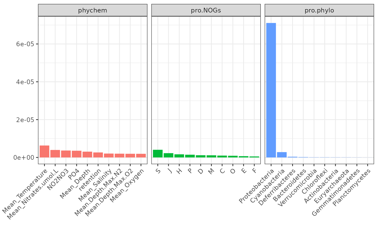
Proteobacteria is the most important variable for the
pro.phylo kernel.
The relative abundance of `Proteobacteria`` is then extracted in each of our 139 samples, and each sample is colored according to the value of this variable in the KPCA projection plot:
selected <- which(TARAoceans$taxonomy[, "Phylum"] == "Proteobacteria")
proteobacteria.per.sample <- apply(TARAoceans$pro.phylo[, selected], 1, sum) /
  apply(TARAoceans$pro.phylo, 1, sum)
colfunc <- colorRampPalette(c("royalblue", "red"))
col.proteo <- colfunc(length(proteobacteria.per.sample))
col.proteo <- col.proteo[rank(proteobacteria.per.sample, ties = "first")]
plotIndiv(kernel.pca.result,
          comp = c(1, 2),
          ind.names = FALSE,
          legend = FALSE,
          col = col.proteo,
          pch = TARAoceans$sample$depth,
          legend.title = "Ocean / Sea",
          title = "Representation of Proteobacteria abundance",
          legend.title.pch = "Depth")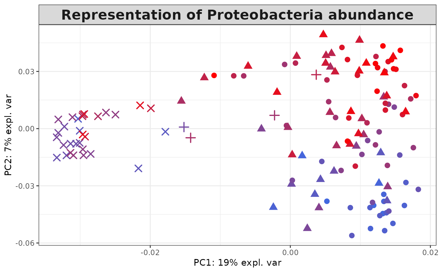
Similarly, the temperature is the most important variable for the
phychem kernel. The temperature values can be displayed on
the kernel PCA projection as follows:
col.temp <- colfunc(length(TARAoceans$phychem[, 4]))
col.temp <- col.temp[rank(TARAoceans$phychem[, 4], ties = "first")]
plotIndiv(kernel.pca.result,
          comp = c(1, 2),
          ind.names = FALSE,
          legend = FALSE,
          col = col.temp,
          pch = TARAoceans$sample$depth,
          legend.title = "Ocean / Sea",
          title = "Representation of mean temperature",
          legend.title.pch = "Depth")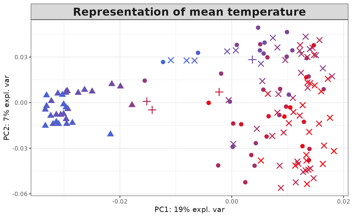
Selecting relevant variables
Here, we use a feature selection approach that does not rely on any
assumption but explicitly takes advantage of the kernel structure in an
unsupervised fashion. The idea is to preserve at best the similarity
structure between samples. These examples requires the installation of
the python modules autograd, scipy,
numpy, and sklearn. See detailed instructions
in the installation vignette or on mixKernel website : http://mixkernel.clementine.wf
have_depend <- reticulate::py_module_available("autograd") &
  reticulate::py_module_available("scipy") &
  reticulate::py_module_available("numpy") &
  reticulate::py_module_available("sklearn")
if (have_depend) {
  ukfs.res <- select.features(TARAoceans$pro.phylo, kx.func = "bray", lambda = 1,
                              keepX = 5, nstep = 1)
  selected <- sort(ukfs.res, decreasing = TRUE, index.return = TRUE)$ix[1:5]
  TARAoceans$taxonomy[selected, ]
}
The select.features function allows to add a structure
constraint to the variable selection. The adjacency matrix of the graph
representing relations between OTUs can be obtained by computing the
Pearson correlation matrix as follows:
library("MASS")
library("igraph")
library("correlationtree")

pro.phylo.alist <- data.frame("names" = colnames(TARAoceans$pro.phylo),
                              t(TARAoceans$pro.phylo))
L <- mat2list(df2mat(pro.phylo.alist, 1))
corr.mat <- as.matrix(cross_cor(L, remove = TRUE))
pro.phylo.graph <- graph_from_adjacency_matrix(corr.mat,
                                               mode = "undirected",
                                               weighted = TRUE)
Lg <- laplacian_matrix(pro.phylo.graph, sparse=TRUE)
if (have_depend) {
  load(file = file.path(system.file(package = "mixKernel"), "loaddata", "Lg.rda"))
  ukfsg.res <- select.features(TARAoceans$pro.phylo, kx.func = "bray",
                               lambda = 1, method = "graph", Lg = Lg, keepX = 5,
                               nstep = 1)

  selected <- sort(ukfsg.res, decreasing = TRUE, index.return = TRUE)$ix[1:5]
  TARAoceans$taxonomy[selected, ]
}
References
Mariette, J. and Villa-Vialaneix, N. (2018). Unsupervised multiple kernel learning for heterogeneous data integration. Bioinformatics, 34(6), 1009-1015.
Zhuang, J., Wang, J., Hoi, S., and Lan, X. (2011). Unsupervised multiple kernel clustering. Journal of Machine Learning Research (Workshop and Conference Proceedings), 20, 129–144.
Lavit, C., Escoufier, Y., Sabatier, R., and Traissac, P. (1994). The act (statis method). Computational Statistics & Data Analysis, 18(1), 97–119.
Session information
## R version 4.5.0 (2025-04-11)
## Platform: x86_64-pc-linux-gnu
## Running under: Ubuntu 24.04.2 LTS
##
## Matrix products: default
## BLAS:   /usr/lib/x86_64-linux-gnu/openblas-pthread/libblas.so.3
## LAPACK: /usr/lib/x86_64-linux-gnu/openblas-pthread/libopenblasp-r0.3.26.so;  LAPACK version 3.12.0
##
## locale:
##  [1] LC_CTYPE=en_US.UTF-8       LC_NUMERIC=C
##  [3] LC_TIME=fr_FR.UTF-8        LC_COLLATE=en_US.UTF-8
##  [5] LC_MONETARY=fr_FR.UTF-8    LC_MESSAGES=en_US.UTF-8
##  [7] LC_PAPER=fr_FR.UTF-8       LC_NAME=C
##  [9] LC_ADDRESS=C               LC_TELEPHONE=C
## [11] LC_MEASUREMENT=fr_FR.UTF-8 LC_IDENTIFICATION=C
##
## time zone: Europe/Paris
## tzcode source: system (glibc)
##
## attached base packages:
## [1] stats     graphics  grDevices utils     datasets  methods   base
##
## other attached packages:
## [1] mixKernel_0.9-2   reticulate_1.42.0 mixOmics_6.30.0   ggplot2_3.5.2
## [5] lattice_0.22-7    MASS_7.3-65
##
## loaded via a namespace (and not attached):
##   [1] mnormt_2.1.1            gridExtra_2.3           permute_0.9-7
##   [4] rlang_1.1.6             magrittr_2.0.3          ade4_1.7-23
##   [7] matrixStats_1.5.0       compiler_4.5.0          mgcv_1.9-3
##  [10] png_0.1-8               systemfonts_1.2.2       vctrs_0.6.5
##  [13] reshape2_1.4.4          quadprog_1.5-8          stringr_1.5.1
##  [16] pkgconfig_2.0.3         crayon_1.5.3            fastmap_1.2.0
##  [19] XVector_0.46.0          labeling_0.4.3          rmarkdown_2.29
##  [22] markdown_2.0            UCSC.utils_1.2.0        ragg_1.4.0
##  [25] purrr_1.0.4             xfun_0.52               zlibbioc_1.52.0
##  [28] cachem_1.1.0            GenomeInfoDb_1.42.3     jsonlite_2.0.0
##  [31] biomformat_1.34.0       rhdf5filters_1.18.0     Rhdf5lib_1.28.0
##  [34] BiocParallel_1.40.0     psych_2.5.3             parallel_4.5.0
##  [37] cluster_2.1.8.1         R6_2.6.1                bslib_0.9.0
##  [40] stringi_1.8.7           RColorBrewer_1.1-3      jquerylib_0.1.4
##  [43] Rcpp_1.0.14             iterators_1.0.14        knitr_1.50
##  [46] IRanges_2.40.1          Matrix_1.7-3            splines_4.5.0
##  [49] igraph_2.1.4            tidyselect_1.2.1        yaml_2.3.10
##  [52] vegan_2.6-10            codetools_0.2-20        tibble_3.2.1
##  [55] plyr_1.8.9              Biobase_2.66.0          withr_3.0.2
##  [58] rARPACK_0.11-0          evaluate_1.0.3          desc_1.4.3
##  [61] survival_3.8-3          Biostrings_2.74.1       pillar_1.10.2
##  [64] phyloseq_1.50.0         corrplot_0.95           foreach_1.5.2
##  [67] stats4_4.5.0            ellipse_0.5.0           generics_0.1.3
##  [70] rprojroot_2.0.4         S4Vectors_0.44.0        munsell_0.5.1
##  [73] scales_1.3.0            glue_1.8.0              tools_4.5.0
##  [76] data.table_1.17.0       RSpectra_0.16-2         fs_1.6.6
##  [79] rhdf5_2.50.2            grid_4.5.0              tidyr_1.3.1
##  [82] ape_5.8-1               colorspace_2.1-1        nlme_3.1-168
##  [85] GenomeInfoDbData_1.2.13 cli_3.6.4               rappdirs_0.3.3
##  [88] textshaping_1.0.0       dplyr_1.1.4             corpcor_1.6.10
##  [91] gtable_0.3.6            sass_0.4.10             digest_0.6.37
##  [94] BiocGenerics_0.52.0     ggrepel_0.9.6           farver_2.1.2
##  [97] LDRTools_0.2-2          htmlwidgets_1.6.4       htmltools_0.5.8.1
## [100] pkgdown_2.1.1           multtest_2.62.0         lifecycle_1.0.4
## [103] here_1.0.1              httr_1.4.7